Reconstruction of Buildings Models Using Handheld Laser Scanner
Abstract
This thesis focuses on the refined 3D point cloud modeling requirements of buildings within the Multi-Aircraft Intelligent Collaborative Test Platform project. By employing handheld Slam scanners to generate 3D point cloud images of buildings, we propose a high-precision and efficient refined modeling method based on point cloud segmentation. This approach addresses existing challenges such as insufficient segmentation accuracy in complex scenarios and difficulties in integrating geometric and semantic information in current methods.
During implementation, we establish a segmentation model that combines multi-feature fusion with deep learning (PointNet++) to enhance segmentation accuracy and robustness in complex environments (e.g., vegetation occlusion and irregular structures). Simultaneously, we design a model reconstruction algorithm with joint geometric-semantic constraints that supplements missing or incomplete external structural features, achieving high-fidelity representation of architectural details including walls, roofs, doors, and windows.
This research provides standardized and reusable methods for refined building point cloud modeling, effectively resolving structural issues like missing and incomplete point cloud data. The system completes fine data acquisition and refined modeling tasks for the near-field portion of the real scene acquisition system, addressing the problem of low scene modeling granularity.
1. Point Cloud Filtering
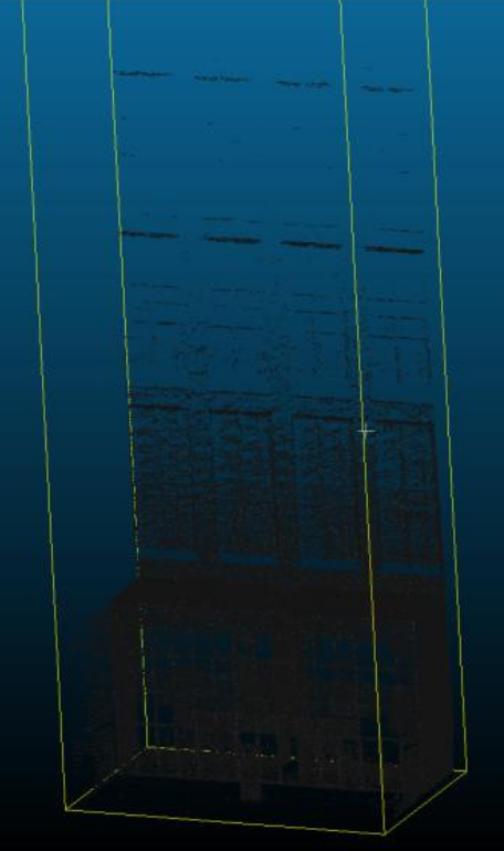
1.1 Data Acquisition
The project utilizes the SLAM-K120 handheld 3D laser scanner, which employs SLAM (Simultaneous Localization and Mapping) technology for real-time positioning and incremental 3D mapping in both indoor and outdoor unknown environments. The scanner obtains spatial 3D information of the surrounding environment while moving, with key specifications including:
- System Accuracy: 1cm precision
- Measurement Distance: 0.05m ~ 120m
- Horizontal Field of View: 360°
- Data Format: LAS format point cloud data
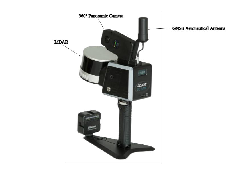
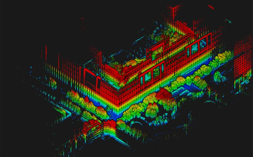
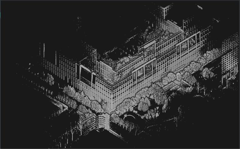
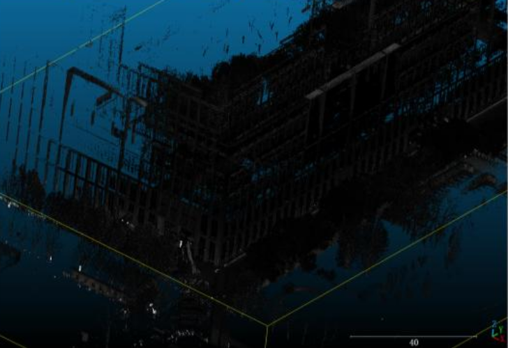
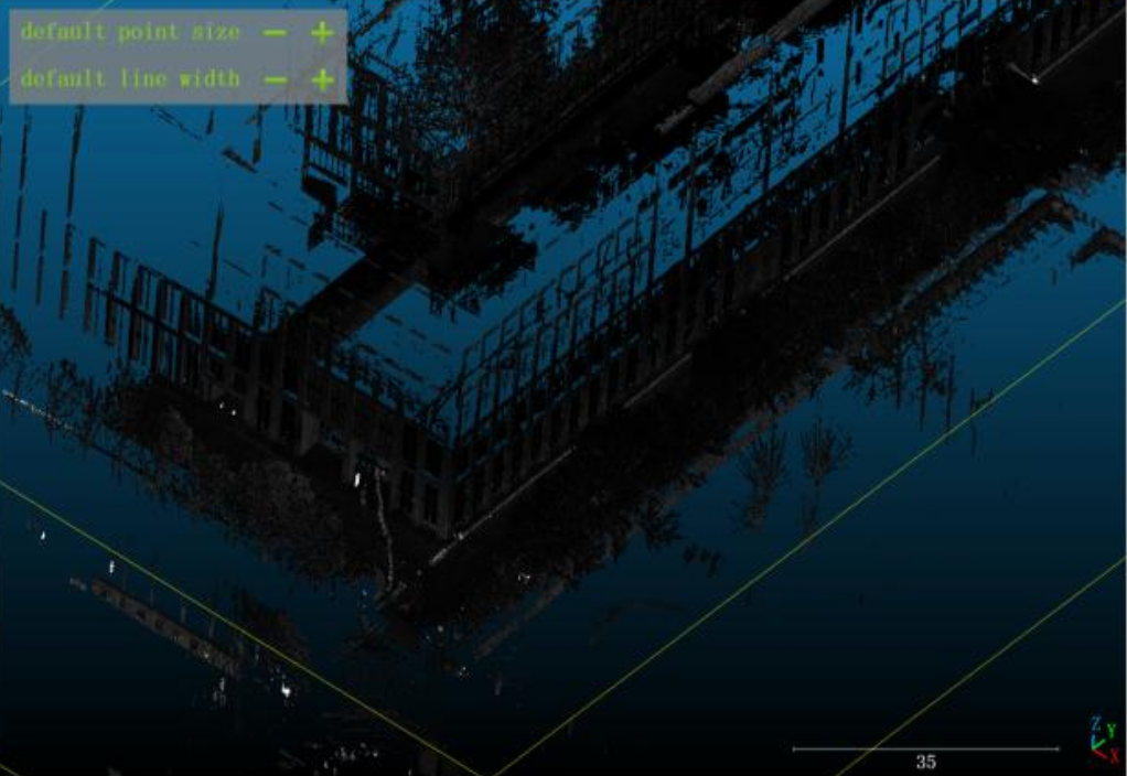
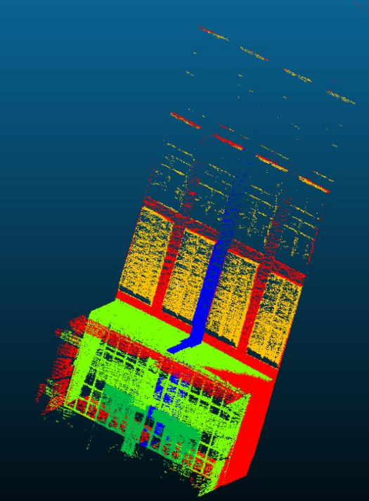
Figure 2.3 shows the point cloud colored by class labels, and Figure 2.4 shows the point cloud colored by elevation. The elevation-based coloring is implemented as follows: each point's elevation (the $z$ coordinate) is mapped to a continuous colormap. First determine the elevation range of the entire point cloud or the region of interest, with a minimum $Z_{\min}$ and maximum $Z_{\max}$. Then normalize each point's elevation by
\[ t = \frac{z - Z_{\min}}{Z_{\max} - Z_{\min}}, \qquad t\in[0,1]. \]
Choose a colormap (for example: blue for low elevation → green → yellow → red for high elevation). The color for a point is obtained by sampling/interpolating the colormap at $t$:
\[ \mathrm{Color}(z) = \mathrm{Colormap}\big(t\big). \]
A simple linear RGB interpolation between a low color $\mathrm{RGB}_{\mathrm{low}}$ and a high color $\mathrm{RGB}_{\mathrm{high}}$ can be written as
\[ \mathrm{RGB}(z) = (1 - t)\,\mathrm{RGB}_{\mathrm{low}} + t\,\mathrm{RGB}_{\mathrm{high}}. \]
More generally, the colormap may be defined by multiple control colors and interpolated piecewise; finally assign the resulting RGB value to each point to produce the elevation-colored point cloud visualization.

1.2 Filtering Algorithms
Statistical Outlier Removal (SOR): To remove isolated noise and measurement outliers, we apply a Statistical Outlier Removal (SOR) filter. For each point i in the point cloud, find its k nearest neighbors and compute the Euclidean distances to those neighbors. Let \(d_{ij}\) denote the distance from point i to its j-th nearest neighbor (\(j=1,\dots,k\)). Let \(N\) be the total
number of points in the cloud. We estimate the global mean distance \(\mu\) and the standard deviation \(\sigma\) over all point-to-neighbor distances as\[ \mu = \frac{1}{N k} \sum_{i=1}^N \sum_{j=1}^k d_{ij}, \qquad \sigma = \sqrt{ \frac{1}{N k} \sum_{i=1}^N \sum_{j=1}^k (d_{ij} - \mu)^2 } \]
For each point i compute its mean neighbor distance
\[ \bar{d}_i = \frac{1}{k} \sum_{j=1}^k d_{ij}. \]
The SOR criterion marks points as outliers when their mean neighbor distance is significantly larger or smaller than the global statistics. Using a user-defined multiplier \(n_{\sigma}\) (often called "nSigma"), the common rule is to remove points that satisfy
\[ \bar{d}_i > \mu + n_{\sigma}\,\sigma \quad\text{or}\quad \bar{d}_i < \mu - n_{\sigma}\,\sigma. \]
In practice the filter is typically applied only to the upper tail (large distances) to remove sparse isolated points; for example, setting \(k=50\) and \(n_{\sigma}=1.0\) removes points whose neighborhood distance is more than one standard deviation above the global mean.
Key parameters include:
- k_neighbors: Number of nearest neighbors used to compute \(\bar{d}_i\) (e.g. 50).
- nSigma (\(n_{\sigma}\)): Standard deviation multiplier controlling the strictness of the filter (e.g. 1.0).
- mode: Upper-tail only or symmetric removal (whether to remove only large-distance outliers or both tails).
In CloudCompare's SOR implementation, the filter exposes a convenient threshold \(d_{\max}\) computed from the global mean and standard deviation of neighbor distances. The maximum allowed distance is often set as
\[ d_{\max} = \bar{d}_i\ + n_{\sigma} \, \sigma. \]
If a point's mean neighbor distance \(\bar{d}_i\) exceeds \(d_{\max}\), it is classified as an outlier and removed. Choosing a small \(n_{\sigma}\) (e.g. 1) makes the filter stricter and removes more points, which may eliminate borderline inliers; choosing a larger \(n_{\sigma}\) (e.g. 2 or 3) relaxes the filter and preserves more points but may leave some noisy points. For large-scale building scans we found that setting \(k=50\) and \(n_{\sigma}=1.0\) gives a good balance between removing isolated noise and keeping structural details.
1.3 Filtering Results
Using CloudCompare software, we processed a building point cloud dataset containing 74,331,016 points. After applying SOR filtering with k=50 and σ=1.0, the cleaned dataset contained 67,921,156 points, effectively removing noise and outliers while preserving structural details. The processing time for this large-scale dataset was approximately 10 minutes.
2. Point Cloud Semantic Segmentation
2.1 Segmentation Architecture
We propose a hybrid network architecture combining local geometric features, global semantic context, and attention mechanisms to optimize segmentation boundary precision in sparse regions. The pipeline consists of:
- Local Geometric Encoding: Dynamic Graph CNN (DGCNN) with EdgeConv operations to capture local feature relationships through k-nearest neighbor graphs.
- Global Context Aggregation: Point Transformer with multi-head self-attention to establish long-range dependencies and capture overall semantic structure.
- Attention Weighting: Channel-spatial dual attention (PAConv) mechanism to enhance key structures (walls, roofs) while suppressing noise.
- Multi-scale Feature Fusion: KPConv-based feature pyramid combining local details with global semantics through skip connections and 1×1 convolutions.
- Boundary Optimization: BADet module for joint geometric edge detection and semantic rule prediction using curvature and normal vector differences.
2.2 Segmentation Results
We performed segmentation experiments on the building-component point clouds described in Section 3.2.1. The training configuration (including number of classes and training hyperparameters) was adjusted to fit the dataset. Training was carried out on a notebook equipped with an NVIDIA GeForce RTX 3060: the model was trained on the training set for 20 hours and further trained on the test set for 10 hours. The resulting segmentation visualization is shown in Figure 5. Scene-level evaluation metrics are reported in Table 3.3. The mean Intersection-over-Union (mIoU) is 0.540, indicating that most building components are correctly recognized, although boundary details may be coarse. The overall accuracy (OA) is 0.836, meaning a high proportion of points are classified correctly.
| Metric | Value |
|---|---|
| mIoU | 0.540 |
| mAcc | 0.639 |
| OA | 0.836 |
3. Point Cloud Refined Modeling
3.1 Challenges
Deep learning segmentation may produce unstable component boundaries, leading to uneven sizing and layout of similar components. Additionally, occlusions from vegetation or other buildings can cause incomplete segmentation results with missing or fragmented features. These issues affect the final modeling quality.
3.2 Component Information Extraction
Building component information is defined by four elements:
- Height and Width: Bounding box dimensions of the component
- Position: Centroid coordinates (average of four vertices) and relative position in the scene
- Spacing: Distance between similar components
| Component info | Symbol | Definition |
|---|---|---|
| Height | H | Distance between top and bottom vertices of the component along the vertical direction |
| Width | W | Distance between left and right vertices of the component along the horizontal direction |
| Position | P | Centroid coordinates of the component |
| Spacing | S | Distance between centroids of neighboring components of the same class |
The extracted information is shown in the table below:
| Component | H (m) | W (m) | Position P (m) |
|---|---|---|---|
| Floor-to-ceiling window | 8.37 | 15.19 | (20.375, -69.365, 4.290) |
| Suspended window 1 | 7.50 | 2.80 | (26.684, -78.603, 13.255) |
| Suspended window 2 | 7.47 | 2.78 | (22.650, -76.680, 13.225) |
| Suspended window 3 | 7.54 | 2.82 | (18.585, -76.813, 13.235) |
| Suspended window 4 | 7.48 | 2.79 | (14.518, -76.920, 13.293) |
| Suspended window 5 | 7.49 | 2.83 | (26.760, -76.683, 21.640) |
| Suspended window 6 | 7.46 | 2.76 | (22.713, -76.678, 21.682) |
| Suspended window 7 | 7.51 | 2.81 | (18.618, -76.873, 21.683) |
| Suspended window 8 | 7.49 | 2.78 | (14.620, -76.985, 21.680) |
| Door | 3.36 | 9.22 | (20.426, -72.575, 1.883) |
| Column | 8.26 | 0.95 | (20.345, -69.540, 4.290) |
K-Means clustering is applied to classify components based on these features, grouping similar windows, doors, and structural elements for standardization and reuse.
According to the component definitions in Table 4.1, a component's height and width depend only on the component itself, while the spacing between components also depends on the component type and its position. Therefore, when classifying component information in this section, we treat components with similar heights and widths as the same class; components that share the same X coordinate are considered to be in the same row; and components that share the same Y coordinate are considered to be in the same column.
Because the height and width of different component types are significantly different in this work, the classification problem can be converted into a two-dimensional K-Means clustering process, where K denotes the number of desired component clusters and each data point's X and Y coordinates represent the component's H and W values respectively. First, the collected (H, W) information is stored as an N×2 NumPy array. Then we train a K-Means model (for example using scikit-learn or a custom script) which outputs K cluster centers and cluster labels — these centers represent the mean feature values for each component class.
For subsequently segmented components, we pass their (H, W) coordinates to the trained K-Means model's predict() function. The algorithm computes the Euclidean distance from the new point to each trained cluster center and assigns the point to the nearest cluster; the corresponding cluster label becomes the component's class. The pseudo-steps are: assemble (H, W) into an N×2 array, fit K-Means to obtain cluster centers and labels, then classify new components by calling predict() and using nearest-center assignment.
predict() function;3.3 Component Regularization and Reuse
Clustering-based Regularization: Components with similar geometric properties are grouped and standardized to a representative prototype, enforcing consistency across the model.
ICP-based Component Reuse: The Iterative Closest Point algorithm aligns segmented component point clouds with templates from a semantic library. Missing or occluded components are completed by:
- Detecting gaps in the building facade through semantic analysis
- Matching expected component types based on surrounding context
- Inserting and aligning template components using ICP registration
- Refining boundaries with geometry-semantic constraints