Mobile Car Projects

Zhi Xing Car I - SLAM Navigation Robot
A comprehensive autonomous navigation robot system integrating SLAM mapping, path planning, voice control, and face recognition. Built on ROS framework with LiDAR-based localization and multi-sensor fusion, achieving robust autonomous navigation and intelligent interaction in indoor environments.
Video
1. Vehicle Kinematics Analysis
This section summarizes the differential-drive vehicle kinematics and control models, including forward/inverse kinematics, relationships between wheel speeds and robot linear/angular velocities, and common trajectory tracking algorithms.
1.1 Odometry & Coordinate Transforms
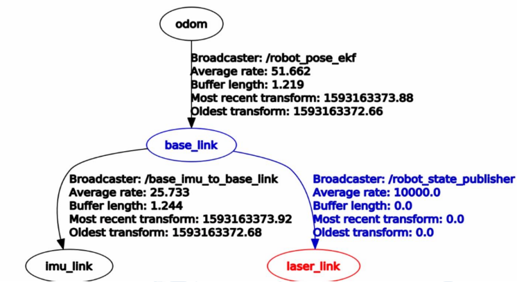
In ROS-based robots the most common frames are map, odom and base_link. The map frame is a fixed, long-term global reference (Z axis up). Because localization may apply discrete corrections when new sensor data arrives, poses expressed in map can occasionally "jump"; this makes map suitable as a global reference but not ideal as a fast local control frame.
The odom frame is a locally-continuous reference produced by dead-reckoning sources (wheel encoders, visual odometry, IMU). odom guarantees smooth, continuous pose updates (no sudden jumps) and is useful as a short-term reference for sensors and controllers, but it accumulates drift and therefore cannot serve as a precise long-term global frame. Typically map and odom start aligned; localization modules compute the transform map → odom (via tf) to correct odometry drift.
Note the distinction between the odom coordinate frame and an /odom topic: the frame is the coordinate reference, whereas the /odom topic commonly publishes the transform from odom to base_link (i.e., the robot pose in the odom frame).
The base_link frame is the robot body frame (usually centered on the platform); the core localization task is estimating base_link's pose in the map frame. Each sensor has its own fixed sensor frame (for example laser or base_laser for a LiDAR), and the transform between that sensor frame and base_link is constant and should be published via tf.
1.2 Kinematic Transformation from Robot Velocity to Motor Speeds
The kinematic model of the differential wheel chassis is established as follows: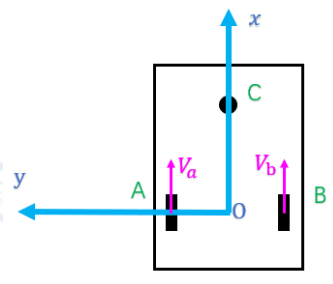
Below are the key points extracted from the image. Let the linear speeds of the two wheels be V_a (wheel A) and V_b (wheel B), and let the track width be 2L. When only one wheel is turning, the contact point of the stationary wheel is the instantaneous center of rotation (ICR), which yields special-case kinematic relations.
1) Only wheel A rotates (wheel B stationary):
$$V_{ox}=\frac{V_a}{2},\quad V_{oy}=0,\quad \dot{\theta}=-\frac{V_a}{2L}$$
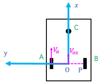
2) Only wheel B rotates (wheel A stationary):
$$ \begin{cases} V_{ox}=\frac{V_b}{2}\\ V_{oy}=0\\ \dot{\theta}=\frac{V_b}{2L} \end{cases} $$
Combining the two special cases gives the general form (superposition of wheel speeds):
$$ \begin{cases} V_{ox}=\tfrac{1}{2}(V_a+V_b)\\ V_{oy}=0\\ \dot{\theta}=\tfrac{1}{2L}(V_b-V_a) \end{cases} $$
Based on the forward kinematic formulation, the corresponding inverse kinematic equations can be directly obtained, establishing the mapping from the robot’s body-frame velocity to each wheel’s linear velocity:
$$ \begin{cases} V_a = V_{ox} + L\,\dot{\theta}\\ V_b = V_{ox} - L\,\dot{\theta} \end{cases} $$
1.3 Kinematic Transformation from Motor Speeds to Robot Displacement
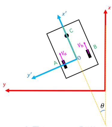
The following summarizes the coordinate transform and velocity relationships illustrated in the diagram above. Let the robot body frame be (x',y') rotated by heading \(\theta\) relative to the global frame (x,y). The coordinate transform from body to global is:
$$x = x'\cos\theta - y'\sin\theta\\ y = x'\sin\theta + y'\cos\theta$$
For the two-wheel differential drive with wheel linear speeds \(V_a\) and \(V_b\) (left/right or labeled in the figure), the derived body-frame velocity components are:
$$ \begin{cases} V_{ox}=\tfrac{1}{2}(V_a+V_b)\cos\phi\\ V_{oy}= -\tfrac{1}{2}(V_a+V_b)\sin\phi\\ \dot{\theta}=\tfrac{1}{2L}(V_b-V_a) \end{cases} $$
This set of equations represents the transformation from the angular velocities of the two motors to the robot’s motion velocity in the global (world) coordinate frame. During odometry computation, the robot’s linear and angular velocities are integrated over each time interval, and the accumulated result yields the current displacement, which corresponds to the data published on the/odom topic.
With this, the derivation of the differential-drive kinematic model is complete.
2. SLAM Navigation Workflow
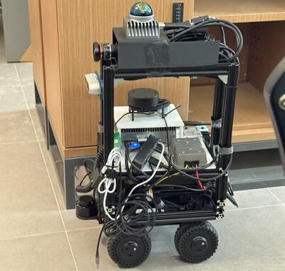
2.1 System Architecture & Hardware Setup
- Computing Platform: On-board computer with ROS Melodic on Ubuntu 18.04
- Sensors: RPLiDAR A1 (360° laser scanner), ReSpeaker voice array, RGB-D camera
- Motor Control: Differential drive system with encoder feedback
- Communication: USB serial communication with custom protocol for motor control
2.2 GMapping Algorithm Based on RBPF
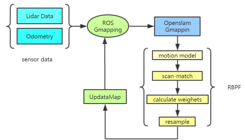
GMapping is a widely used SLAM (Simultaneous Localization and Mapping) algorithm based on the Rao-Blackwellized Particle Filter (RBPF) framework.
It factorizes the full SLAM posterior into two parts: the robot trajectory estimation and the map estimation.
$$ p(x_{1:t}, m \mid z_{1:t}, u_{1:t-1}) = p(m \mid x_{1:t}, z_{1:t}) \, p(x_{1:t} \mid z_{1:t}, u_{1:t-1}) $$
where:
- \(x_{1:t}\): the robot trajectory up to time \(t\);
- \(m\): the map of the environment;
- \(z_{1:t}\): the sequence of sensor measurements (e.g., LiDAR scans);
- \(u_{1:t-1}\): the sequence of control inputs (odometry).
1. Improved Proposal Distribution
In traditional FastSLAM 1.0, the proposal distribution for sampling new particle poses only depends on the motion model:
$$p(x_t\mid x_{t-1}, u_t)$$
This approach suffers from high uncertainty due to odometry drift and noise, often causing particle degeneracy — only a few particles have significant weights.
GMapping improves this by incorporating the current observation \(z_t\) into the proposal distribution:
$$p(x_t\mid x_{t-1}, u_t, z_t)$$
Key idea: combining motion and observation information corrects the motion-model prediction using the latest laser scan, reducing uncertainty of sampled particles.
Implementation steps:
- For each particle \(i\), predict a set of pose candidates using the motion model.
- Evaluate each candidate by computing the likelihood \(p(z_t\mid x_t^{(i)}, m_{t-1}^{(i)})\) through scan matching.
- Approximate this likelihood as a Gaussian distribution around the best-matched pose.
- Sample the new particle pose from this corrected Gaussian proposal.
The particle weight update becomes:
$$w_t^{(i)} \propto w_{t-1}^{(i)} \dfrac{p(z_t\mid x_t^{(i)}, m_{t-1}^{(i)})\, p(x_t^{(i)}\mid x_{t-1}^{(i)}, u_t)}{q(x_t^{(i)}\mid x_{t-1}^{(i)}, u_t, z_t)}$$
Effect:
- Reduces particle dispersion and improves localization accuracy.
- Requires fewer particles (typically tens instead of hundreds).
- Increases robustness against odometry drift.
2. Selective Resampling
In a standard particle filter, resampling is performed at every iteration to prevent weight degeneracy. Frequent resampling can cause sample impoverishment, reducing particle diversity and potentially leading to local minima. GMapping uses selective resampling:
Only perform resampling when the effective sample size \(N_{\text{eff}}\) falls below a threshold.
The effective sample size is defined as:
$$N_{\text{eff}} = \dfrac{1}{\sum_{i=1}^{N} (w_t^{(i)})^2}$$
When \(N_{\text{eff}} < N_{\text{threshold}}\) (typically \(N/2\) or \(N/3\)), resampling is triggered.
Benefits:
- Maintains particle diversity.
- Avoids unnecessary resampling when the weight distribution is stable.
- Improves convergence speed and map consistency.
2.3 Navigation
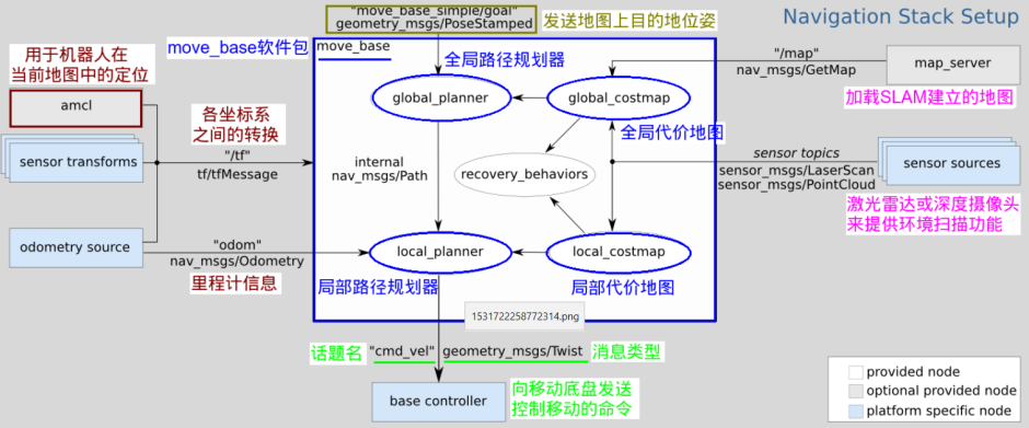 At the core of the navigation system lies the
 move_base node, which integrates inputs from odometry, robot pose estimation, and map data.
This node performs both global planning and local planning: the global planner generates an overall path to the target, while the local planner continuously adjusts the trajectory in response to environmental changes, thus achieving autonomous obstacle avoidance during navigation.
1.Localization
Below is the standard MCL (Monte Carlo Localization) algorithm presented as pseudocode. Variables: \(\mathcal{X}_{t-1}\) is the particle set at time \(t-1\), \(u_t\) the control input, \(z_t\) the current observation, and \(m\) the map.
AMCL (Adaptive Monte Carlo Localization) is a particle-filter-based method for robot localization. Its objective is to estimate the robot pose over time from sensor measurements and control inputs. We denote the robot pose at time \(t\) by \(x_t\); the control (odometry) input applied between time \(t-1\) and \(t\) by \(u_t\); and the sensor observation at time \(t\) by \(z_t\). When referring to histories we use the shorthand sequences \(x_{1:t}\), \(u_{1:t}\) and \(z_{1:t}\). Using the Bayes filter formulation, the posterior can be written as:
$$ p(x_t\mid z_{1:t}, u_{1:t}) = \eta\; p(z_t\mid x_t)\; p(x_t\mid z_{1:t-1}, u_{1:t}) $$
Here the prediction (motion update) step is given by the Chapman–Kolmogorov equation:
$$ p(x_t\mid z_{1:t-1}, u_{1:t}) = \int p(x_t\mid x_{t-1}, u_t)\; p(x_{t-1}\mid z_{1:t-1}, u_{1:t-1})\, dx_{t-1}. $$
The measurement update then incorporates the current observation \(z_t\) via the likelihood \(p(z_t\mid x_t)\), and \(\eta\) is a normalizing constant.
AMCL approximates the posterior with a set of weighted particles \(\{x_t^{(i)}, w_t^{(i)}\}_{i=1}^M\). The particle filter loop typically performs:
Here, M denotes the number of particles.
- Prediction: sample a new pose for each particle from the motion model \(x_t^{(i)} \sim p(x_t\mid x_{t-1}^{(i)}, u_t)\).
- Update: compute the importance weight using the observation likelihood, e.g. \(w_t^{(i)} \propto w_{t-1}^{(i)}\; p(z_t\mid x_t^{(i)})\), then normalize the weights.
- Resample: when particle degeneracy is detected, draw a new particle set according to the normalized weights.
$$ w_t^{(i)} \propto w_{t-1}^{(i)}\; p(z_t\mid x_t^{(i)}) $$
A common metric to decide whether to resample is the Effective Sample Size (ESS):
$$ N_{\text{eff}} = \dfrac{1}{\sum_{i=1}^{M} (w_t^{(i)})^2} $$
When \(N_{\text{eff}}\) falls below a chosen threshold (for example \(M/2\)), resampling is performed. AMCL uses adaptive resampling strategies (and can vary the number of particles) based on ESS to balance computational cost and localization accuracy. This adaptive behavior helps maintain robustness in real-time robot localization.
2. move_base
Global path planning is primarily used to generate an optimal route from the robot’s current position to the target within a known map, while local path planning focuses on real-time motion adjustment along the global path to ensure obstacle avoidance in partially unknown environments.The move_base stack commonly uses costmaps to represent the environment and perform planning. In ROS, the costmap_2d package generates different costmap layers on top of the base map to support both local and global planners. Typical layers include:
- Static Map Layer: a largely unchanging layer (usually produced by SLAM) representing the static environment used for global planning.
- Obstacle Map Layer: a dynamic layer that records obstacles detected by sensors (e.g., LiDAR); used by local planners to avoid newly observed obstacles.
- Inflation Layer: expands occupied cells outward to create a safety margin around obstacles, preventing the robot from planning paths too close to obstacles.
- Other Layers: additional layers can be implemented as plugins (for example, Social Costmap Layer, Range Sensor Layer, etc.) to provide specialized behavior.
3. Common Global and Local Path Planners
The navigation stack typically separates planning into global planners (produce a full path on a known map) and local planners (reactive, operate in velocity space to follow the global path while avoiding obstacles).
Global Planners
- A* (A-star): A graph-search algorithm that combines cost-to-come and heuristics to find the shortest path from start to goal. A* expands nodes by minimizing the estimated total cost (g + h), and is widely used for grid-based global planning.
- Dijkstra: A classic single-source shortest-path algorithm. Dijkstra expands the frontier by always selecting the node with the smallest current cost from the start, guaranteeing an optimal shortest path in graphs with non-negative edge weights.
- RRT (Rapidly-exploring Random Trees): A sampling-based planner that rapidly grows a tree in the configuration space by random sampling. RRT is effective in high-dimensional or complex environments to quickly find a feasible path, though the paths often require post-processing or smoothing.
Local Planners
- DWA (Dynamic Window Approach): A local planner that searches in the robot's velocity space for collision-free, dynamically-feasible velocity commands. DWA considers the robot's kinematic and dynamic limits, samples candidate linear/angular velocities, and scores them by progress toward the global path and obstacle clearance.
- Sample the robot's control space (linear and angular velocities) within dynamic constraints (dx, dy, dtheta).
- For each sampled velocity, forward-simulate the resulting short-duration trajectory from the current state to predict where the robot would be after a small time step.
- Evaluate each forward-simulated trajectory using objective terms: obstacle proximity (collision checking), closeness to the global path/goal, and dynamic feasibility (respecting velocity/acceleration limits). Discard trajectories that violate constraints or are clearly infeasible.
- Select the highest-scoring trajectory and publish the corresponding velocity command to the base controller.
- TEB (Timed Elastic Band): An optimization-based local planner that represents the trajectory as a sequence of time-stamped poses (an elastic band). By optimizing both timing and spatial configuration under kinodynamic constraints, TEB produces smooth, feasible local trajectories that can respect obstacle avoidance and dynamic limits.
References
- G. Grisetti, C. Stachniss, and W. Burgard, "Improving grid-based SLAM with Rao-Blackwellized particle filters by adaptive proposals and selective resampling," in Proc. IEEE Int. Conf. Robotics and Automation (ICRA), 2005, pp. 2432–2437. [PDF]
- Z. Wang, "GMapping and AMCL summary," CSDN Blog, 2024. [https://blog.csdn.net/m0_55202222/article/details/131065091]
Zhi Xing Car II
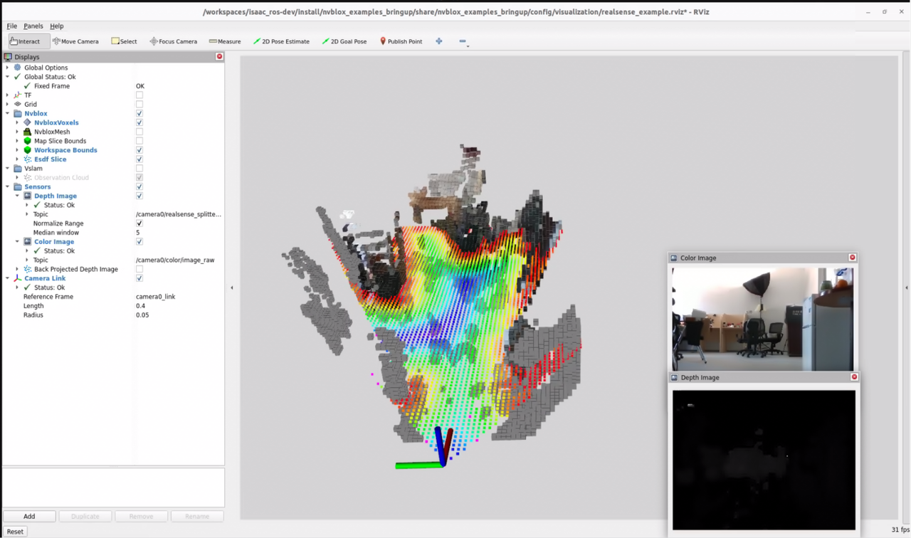
We designed and deployed a SLAM system on NVIDIA Jetson, integrating 2D LiDAR and RealSense D435 for robust multi-sensor fusion. Implemented Google Cartographer for high-accuracy 2D localization and mapping, and extended to 3D ESDF-based mapping for precise environmental reconstruction and optimized path planning in real-world navigation tasks.
1. Simulation
2. NVBlox 3D Reconstruction
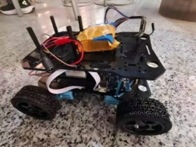
Auto-tracking Car
We used OpenCV to rectify the camera-captured map and extract obstacle coordinates for path planning. Based on the map, we designed an efficient motion planning algorithm using A* search algorithm, enabling the car to avoid randomly positioned obstacles. Then we implemented a PID controller for precise speed and steering control, ensuring smooth navigation.
Video
1. Rectify the Camera-captured Map
- image_transformer rectifies the oblique map captured by the camera to obtain a bird's-eye (top-down) view map.
- Image enhancement: use
convertScaleAbsto increase contrast (alpha=1.5) so colors are easier to distinguish. - Color space conversion: convert BGR to HSV; HSV is more robust to illumination changes under varying lighting.
2. Extract Obstacle Coordinates
Sampling strategy (9x9 grid center sampling):
i = j = 40
tiles = []
while i < 720:
    while j < 720:
        tiles.append(hsv2color(hsv[i, j]))  # sample every 80 pixels at the center of each grid cell
        j += 80
    j = 40
    i += 80

# Start from (40, 40), step = 80 pixels
# Cover 720x720 image → 9x9 = 81 tiles
Color to state mapping for each sampled grid center:
- 0: black (obstacle)
- 2: blue (treasure)
- 3: green (exit)
- 4: yellow (start)
3. Path Planning
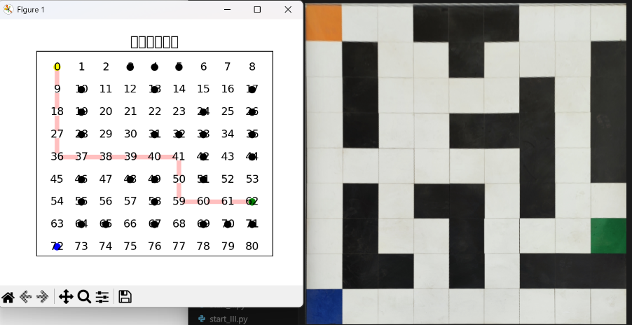
Graph construction logic:
# Build graph
G = nx.Graph()
for target in range(0, 81):
  up = target - 9
  down = target + 9
  left = target - 1
  right = target + 1

  # obstacle weight = 1000 (penalize but not forbidden), passable weight = 1
  if up >= 0:
    if tiles[up] == 0:
      G.add_weighted_edges_from([(target, up, 1000)])
    else:
      G.add_weighted_edges_from([(target, up, 1)])
  if down < 81:
    if tiles[down] == 0:
      G.add_weighted_edges_from([(target, down, 1000)])
    else:
      G.add_weighted_edges_from([(target, down, 1)])
  # ensure left/right do not cross row boundaries
  if left // 9 == target // 9:
    if tiles[left] == 0:
      G.add_weighted_edges_from([(target, left, 1000)])
    else:
      G.add_weighted_edges_from([(target, left, 1)])
  if right // 9 == target // 9:
    if tiles[right] == 0:
      G.add_weighted_edges_from([(target, right, 1000)])
    else:
      G.add_weighted_edges_from([(target, right, 1)])

# Node indices: 0-80, row-major from top-left to bottom-right
# Weight strategy: obstacle=1000 (penalty), normal=1
# Two-stage routing:
find_treasure = nx.dijkstra_path(G, source=start, target=treasure)
find_exit = nx.dijkstra_path(G, source=treasure, target=destination)
Using A* (recommended for grid maps)
A* uses a heuristic to guide the search. For a 2D grid, the Manhattan distance is a simple admissible heuristic:
def manhattan(u, v):
    ux, uy = divmod(u, 9)
    vx, vy = divmod(v, 9)
    return abs(ux - vx) + abs(uy - vy)

# Using networkx's A* (assuming G is built as above and weights represent cost):
path_to_treasure = nx.astar_path(G, source=start, target=treasure, heuristic=manhattan, weight='weight')
path_to_exit = nx.astar_path(G, source=treasure, target=destination, heuristic=manhattan, weight='weight')